Distributed Deep Learning Pipelines with PySpark and Keras

An easy approach to data pipelining using PySpark and performing distributed deep learning with Keras.

Last updated on Oct 21, 2020 8 min read

Deep learning has achieved great success in many areas recently. It has attained state-of-the-art performance in applications ranging from image classification and speech recognition to time series forecasting. The key success factors of deep learning are – big volumes of data, flexible models and ever-growing computing power. With the increase in the number of parameters and training data, it is observed that the performance of deep learning can be improved dramatically. However, when models and training data get big, they may not fit in the memory of a single CPU or GPU machine, and thus model training could become slow. One of the approaches to handle this challenge is to use large-scale clusters of machines to distribute the training of deep neural networks (DNNs).

In this notebook, we use PySpark [1], Keras [2], and Elephas [3] Python libraries to build a deep learning pipeline that runs on Spark.

Step 1: Import Libraries

# Spark Session, Pipeline, Functions, and Metrics
from pyspark import SparkContext, SparkConf
from pyspark.sql import SQLContext
from pyspark.ml.feature import OneHotEncoderEstimator, StringIndexer, StandardScaler, VectorAssembler
from pyspark.ml import Pipeline
from pyspark.sql.functions import rand
from pyspark.mllib.evaluation import MulticlassMetrics

# Keras / Deep Learning
from keras.models import Sequential
from keras.layers.core import Dense, Dropout, Activation
from keras import optimizers, regularizers
from keras.optimizers import Adam

# Elephas for Deep Learning on Spark
from elephas.ml_model import ElephasEstimator

Step 2: Start Spark Session

You can set a name for your project using setAppName() and also set how many workers you want. Just a warning, if your data is not very large, then distributing the work might actually be less useful and provide worse results.

# Spark Session
conf = SparkConf().setAppName('Spark DL Pipeline').setMaster('local[6]')
sc = SparkContext(conf=conf)
sql_context = SQLContext(sc)

Step 3: Load and Preview Data

Firstly, we load the data. The inferSchema parameter helps to identify the feature types when loading in the data.

# Load Data to Spark Dataframe
df = sql_context.read.csv('/bank.csv',
                    header=True,
                    inferSchema=True)

After loading the data, we can see the schema and the various feature types.

# View Schema
df.printSchema()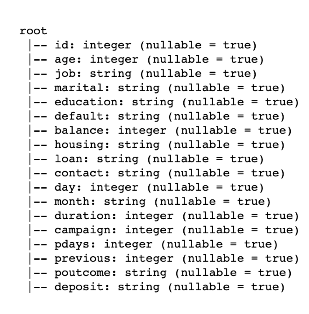

Moreover, if you want to convert the spark dataframe into a pandas dataframe to perform several manipulations, you can use the function toPandas().

# Preview Dataframe
df.limit(5).toPandas()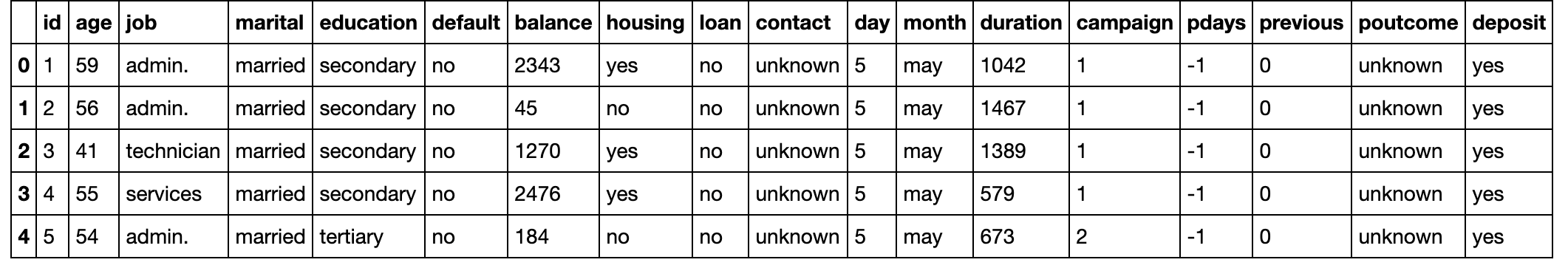

# Drop Unnecessary Features (Day and Month)
df = df.drop('day', 'month')

Step 4: Create the Spark Data Pipeline

Now, we create the pipeline using PySpark. This essentially takes your data and, will do the transformations and vectorizing so it is ready for modeling. For more information, read the documentation Extracting, transforming and selecting features.

Below is a helper function to select from the numeric features which ones to standardize based on the kurtosis or skew of that feature. The current defaults for upper_skew and lower_skew are just general guidelines, but you can modify the upper and lower skew as desired.

# Helper function to select features to scale given their skew
def select_features_to_scale(df=df, lower_skew=-2, upper_skew=2, dtypes='int32', drop_cols=['']):
    
    # Empty Selected Feature List for Output
    selected_features = []
    
    # Select Features to Scale based on Inputs ('in32' type, drop 'ID' columns or others, skew bounds)
    feature_list = list(df.toPandas().select_dtypes(include=[dtypes]).columns.drop(drop_cols))
    
    # Loop through 'feature_list' to select features based on Kurtosis / Skew
    for feature in feature_list:

        if df.toPandas()[feature].kurtosis() < -2 or df.toPandas()[feature].kurtosis() > 2:
            
            selected_features.append(feature)
    
    # Return feature list to scale
    return selected_features

The feature selection by type can be done with the function spark_df.toPandas().select_dtypes(include=['object']).columns), which returns a list of all the columns in your spark dataframe that are object or string type. For this small dataset, the feature selection is done manually with cat_features, num_features, and label.

After selecting features, we create an empty list called stages. This will contain every step that the data pipeline needs to complete all transformations within our pipeline. Then, we index and encode each categorical feature from our list cat_features using one-hot encoding (OHE). One-hot encoding maps a categorical feature, represented as a label index, to a binary vector with at most a single one-value indicating the presence of a specific feature value from among the set of all feature values. This encoding allows algorithms which expect continuous features, such as Logistic Regression, to use categorical features. For string type input data, it is common to encode categorical features using StringIndexer.

Next, we move on to scaling the numeric variables using the select_features_to_scale helper function. We vectorize and standardize the features using VectorAssembler and StandardScaler, respectively.

The last step is just assembling all our features into a single vector. We find the numeric features from the list num_features that were not scaled by just using the difference between our unscaled_features list and the original list of numeric features num_features. Then, we assemble or vectorize all the categorical OHE features and numeric features. We add in the scaled_features to our assembled_inputs to get a final and single vector of features for our modeling.

# Spark Pipeline
cat_features = ['job', 'marital', 'education', 'default', 'housing', 'loan', 'contact', 'poutcome']
num_features = ['age','balance','duration','campaign','pdays','previous']
label = 'deposit'

# Pipeline Stages List
stages = []

# Loop for StringIndexer and OHE for Categorical Variables
for features in cat_features:
    
   # Index Categorical Features
  string_indexer = StringIndexer(inputCol=features, outputCol=features + "_index")
    
  # One Hot Encode Categorical Features
  encoder = OneHotEncoderEstimator(inputCols=[string_indexer.getOutputCol()], outputCols=[features + "_class_vec"])
 
  # Append Pipeline Stages
  stages += [string_indexer, encoder]
    
# Index Label Feature
label_str_index =  StringIndexer(inputCol=label, outputCol="label_index")

# Scale Feature: Select the Features to Scale using helper 'select_features_to_scale' function above and Standardize 
unscaled_features = select_features_to_scale(df=df, lower_skew=-2, upper_skew=2, dtypes='int32', drop_cols=['id'])

unscaled_assembler = VectorAssembler(inputCols=unscaled_features, outputCol="unscaled_features")

scaler = StandardScaler(inputCol="unscaled_features", outputCol="scaled_features")

stages += [unscaled_assembler, scaler]

# Create list of Numeric Features that Are Not Being Scaled
num_unscaled_diff_list = list(set(num_features) - set(unscaled_features))

# Assemble or Concat the Categorical Features and Numeric Features
assembler_inputs = [feature + "_class_vec" for feature in cat_features] + num_unscaled_diff_list

assembler = VectorAssembler(inputCols=assembler_inputs, outputCol="assembled_inputs") 

stages += [label_str_index, assembler]

# Assemble Final Training Data of Scaled, Numeric, and Categorical Engineered Features
assembler_final = VectorAssembler(inputCols=["scaled_features","assembled_inputs"], outputCol="features")

stages += [assembler_final]

We can see all the steps within our pipeline by looking at our stages list that we've been sequentially adding.

stages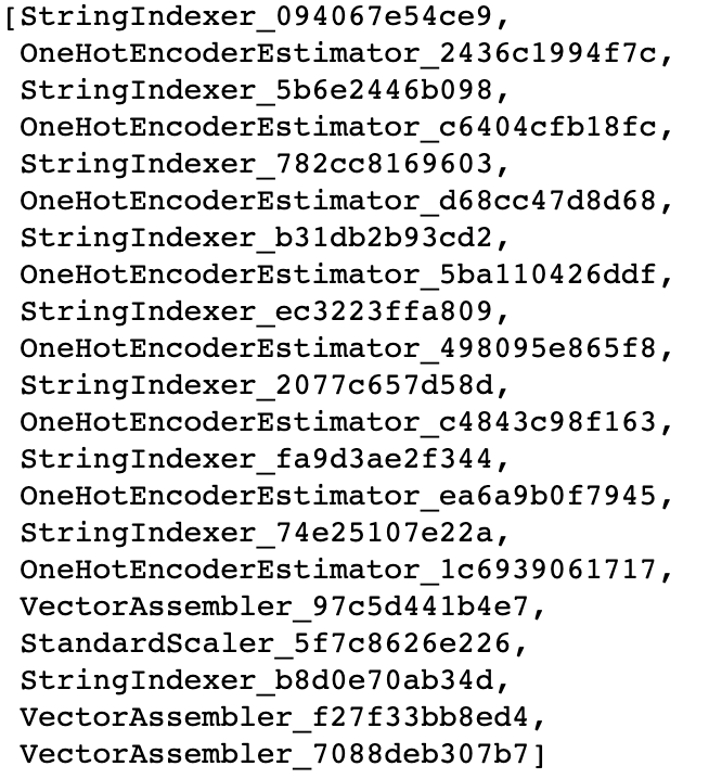

Step 5: Run Data Through the Spark Pipeline

# Set Pipeline
pipeline = Pipeline(stages=stages)

# Fit Pipeline to Data
pipeline_model = pipeline.fit(df)

# Transform Data using Fitted Pipeline
df_transform = pipeline_model.transform(df)

# Preview Newly Transformed Data
df_transform.limit(5).toPandas()

Step 6: Final Data Preparation before Deep Learning Model

Before the modeling step, we create a PySpark dataframe that only contains 2 vectors from the recently transformed dataframe. In particular, we only need the features (X) and label_index (y) features for modeling.

# Select only 'features' and 'label_index' for Final Dataframe
df_transform_fin = df_transform.select('features','label_index')

# Preview Dataframe
df_transform_fin.limit(5).toPandas()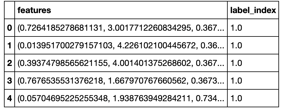

Finally, we shuffle our dataframe and then split the data into train and test sets.

# Shuffle Data
df_transform_fin = df_transform_fin.orderBy(rand())

# Split Data into Train / Test Sets
train_data, test_data = df_transform_fin.randomSplit([.8, .2])

Step 7: Build a Deep Learning Model

This step builds a basic deep learning model using Keras. First, we need to determine the number of classes as well as the number of inputs from our data so we can plug those values into our Keras deep learning model.

# Number of Classes
nb_classes = train_data.select("label_index").distinct().count()

# Number of Inputs or Input Dimensions
input_dim = len(train_data.select("features").first()[0])

Next, we create a basic deep learning model. Using the model = Sequential() feature from Keras, it's easy to simply add layers and build a deep learning model the all the desired settings (# of units, dropout %, regularization - l2, activation functions, etc.).

# Set up Deep Learning Model / Architecture
model = Sequential()
model.add(Dense(256, input_shape=(input_dim,), activity_regularizer=regularizers.l2(0.01)))
model.add(Activation('relu'))
model.add(Dropout(rate=0.3))
model.add(Dense(256, activity_regularizer=regularizers.l2(0.01)))
model.add(Activation('relu'))
model.add(Dropout(rate=0.3))
model.add(Dense(nb_classes))
model.add(Activation('sigmoid'))
model.compile(loss='binary_crossentropy', optimizer='adam')

Once the model is built, we can view the architecture.

# Model Summary
model.summary()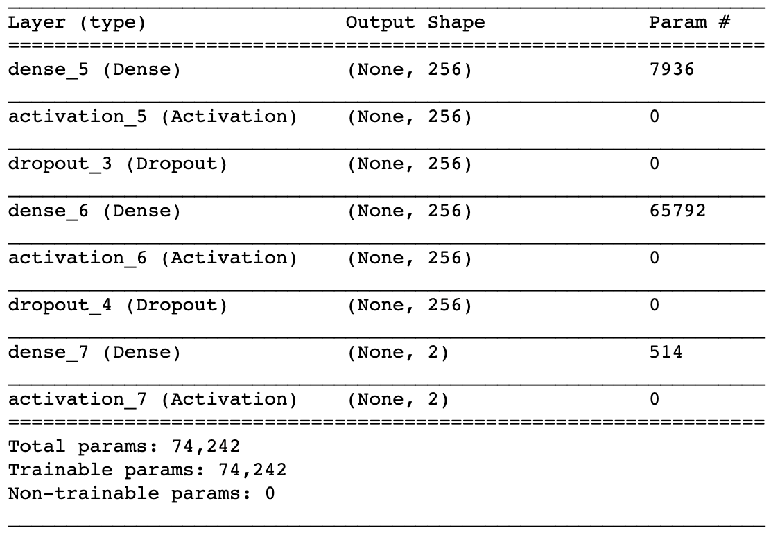

Step 8: Distributed Deep Learning

We run the model on Spark using Elephas. The first thing we do with Elephas is create an estimator similar to some of the PySpark pipeline items above. We can set the optimizer settings right from Keras optimizer function and then pass that to our Elephas estimator. Then, within the Elephas estimator, you specify a variety of items: features column, label column, # of epochs, batch size for training, validation split of your training data, loss function, metric, etc.

# Set and Serialize Optimizer
optimizer_conf = optimizers.Adam(lr=0.01)
opt_conf = optimizers.serialize(optimizer_conf)

# Initialize SparkML Estimator and Get Settings
estimator = ElephasEstimator()
estimator.setFeaturesCol("features")
estimator.setLabelCol("label_index")
estimator.set_keras_model_config(model.to_yaml())
estimator.set_categorical_labels(True)
estimator.set_nb_classes(nb_classes)
estimator.set_num_workers(1)
estimator.set_epochs(25) 
estimator.set_batch_size(64)
estimator.set_verbosity(1)
estimator.set_validation_split(0.10)
estimator.set_optimizer_config(opt_conf)
estimator.set_mode("synchronous")
estimator.set_loss("binary_crossentropy")
estimator.set_metrics(['acc'])

Step 9: Distributed Deep Learning Pipeline and Results

Now that are deep learning model is to be run on Spark using Elephas, we can pipeline line it exactly how we did above using Pipeline().

I create another helper function below, called dl_pipeline_fit_score_results, that takes the deep learning pipeline dl_pipeline and then does all the fitting, transforming, and prediction on both the train and test data sets. It also outputs the accuracy for both data sets and their confusion matrices.

# Create Deep Learning Pipeline
dl_pipeline = Pipeline(stages=[estimator])

def dl_pipeline_fit_score_results(dl_pipeline=dl_pipeline,
                                  train_data=train_data,
                                  test_data=test_data,
                                  label='label_index'):
    
    fit_dl_pipeline = dl_pipeline.fit(train_data)
    pred_train = fit_dl_pipeline.transform(train_data)
    pred_test = fit_dl_pipeline.transform(test_data)
    
    pnl_train = pred_train.select(label, "prediction")
    pnl_test = pred_test.select(label, "prediction")
    
    pred_and_label_train = pnl_train.rdd.map(lambda row: (row[label], row['prediction']))
    pred_and_label_test = pnl_test.rdd.map(lambda row: (row[label], row['prediction']))
    
    metrics_train = MulticlassMetrics(pred_and_label_train)
    metrics_test = MulticlassMetrics(pred_and_label_test)
    
    print("Training Data Accuracy: {}".format(round(metrics_train.precision(),4)))
    print("Training Data Confusion Matrix")
    display(pnl_train.crosstab('label_index', 'prediction').toPandas())
    
    print("\nTest Data Accuracy: {}".format(round(metrics_test.precision(),4)))
    print("Test Data Confusion Matrix")
    display(pnl_test.crosstab('label_index', 'prediction').toPandas())

Let's use our new deep learning pipeline and helper function on both data sets and test our results!

dl_pipeline_fit_score_results(dl_pipeline=dl_pipeline,
                              train_data=train_data,
                              test_data=test_data,
                              label='label_index')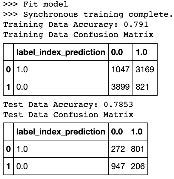

References

[1] PySpark https://spark.apache.org/docs/latest/api/python/index.html.

[2] Keras https://keras.io/.

[3] Elephas https://github.com/maxpumperla/elephas.